
Data Preprocessing for Machine Learning
From messy real-world data to model-ready inputs — an intuitive exploration of Feature Engineering, Missing Values, Scaling, and Normalization through child-inspired analogies

Introduction
Most ML tutorials jump straight into models and algorithms. But here's the thing no one tells beginners: the model is not where the magic happens. The data preparation is.
Think of it this way. You wouldn't hand a toddler a jigsaw puzzle with missing pieces, warped edges, and pieces from three different puzzles mixed, and then blame the toddler for not solving it. That's exactly what happens when we feed raw, messy data into a machine learning model and wonder why it performs terribly.
Data preprocessing is the act of preparing raw data so a model can actually make sense of it. It covers everything from creating useful features to handling gaps in the data to making sure numbers play fair with each other. In this piece, we’ll walk through four pillars of preprocessing — Feature Engineering, Handling Missing Values, Scaling, and Normalization. Not as dry mathematical procedures, but as intuitive steps you’ve already seen in how children learn to organize their world.
By the end, you won’t just know what these terms mean. You’ll understand why they exist, when they matter, and what breaks when you skip them.
Why Preprocessing Matters
A machine learning model is only as good as the data it receives.
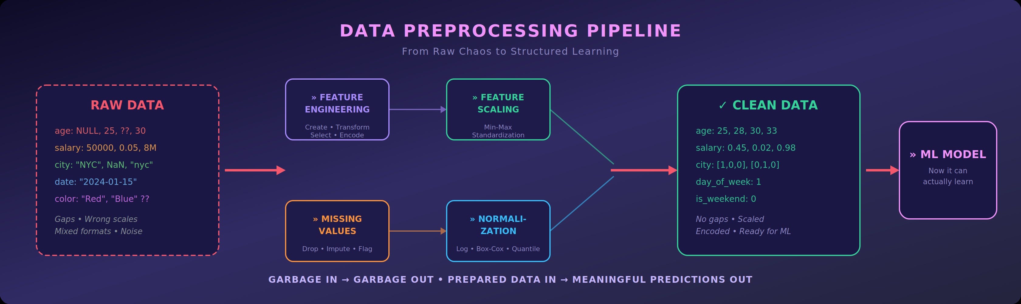
Raw data from the real world is messy. It has gaps. It has inconsistencies. Some numbers are in the thousands, others are tiny decimals. Some information is buried inside other information and needs to be extracted before it becomes useful.
Preprocessing is the bridge between raw chaos and structured learning.
The Four Pillars of Data Preprocessing
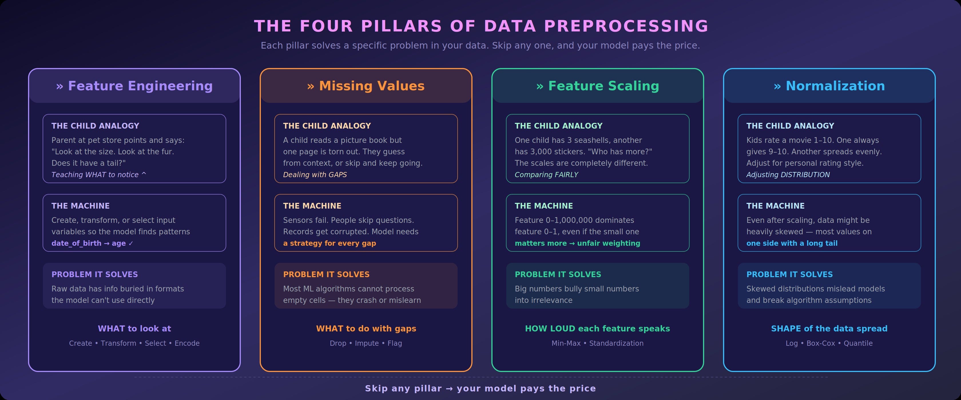
Each pillar solves a specific problem in your data. Skip any one of them, and your model pays the price.
1. Feature Engineering:
Teaching the Machine What to Notice
The Child: A child walks into a pet store. They see animals everywhere. But their parents point and say, “Look at the size. Look at the fur. Does it have a tail?” The parent isn’t changing the animals; they’re teaching the child what to pay attention to.
The Machine: Raw data often contains information, but not in a form the model can use directly. Feature engineering is the process of creating, transforming, or selecting the right input variables (features) so the model can actually find patterns.
Why it matters: A column called “date_of_birth” is useless to a model predicting insurance risk. But a new column called “age” was derived from that date? Now the model has something it can work with.

What Feature Engineering Looks Like in Practice
Creating new features from existing ones: You have a “timestamp” column. You extract “hour_of_day”, “day_of_week”, and “is_weekend”. Suddenly, a model predicting restaurant traffic has useful signals instead of a raw timestamp it can’t interpret.
Combining features: You have “house_length” and “house_width”. Neither alone tells the full story. Multiply them to get “house_area”, a single feature that captures what two couldn’t.
Encoding categories: A column says “Red”, “Blue”, “Green”. A model doesn’t speak English. You convert these to numbers the model can process; one-hot encoding turns “Red” into [1, 0, 0], “Blue” into [0, 1, 0], and so on.
The Takeaway: Feature engineering is the art of translating human knowledge into a language the model can learn from. The model finds patterns, but you decide what it gets to look at.
2. Handling Missing Values:
Filling in the Gaps
The Child: A child is reading a picture book, and one page is torn out. They don’t throw away the entire book. They might guess what happened on that page based on the story before and after. Or they skip it and keep reading.
The Machine: Real-world datasets almost always have missing values. Sensors fail. People skip survey questions. Records get corrupted. The model needs a strategy: fill the gap, remove the gap, or flag the gap.
Why it matters: Most ML algorithms cannot process empty cells. If you don’t handle missing values, your model either crashes or silently learns the wrong thing.

The Three Strategies for Missing Data
Strategy 1 — Remove it (Drop): If only a tiny fraction of your data has gaps, sometimes the simplest move is to drop those rows. Like a child skipping the torn page, you lose a little, but the rest of the story still makes sense. Risk: If too many rows have gaps, you lose valuable data.
Strategy 2 — Fill it (Impute): Replace the missing value with something reasonable. The most common approaches: use the mean (average) for numerical data, the mode (most frequent value) for categorical data, or the median if your data has extreme outliers. Like the child guessing what happened on the missing page based on context.
Strategy 3 — Flag it (Indicator): Create a new column that says “this value was missing” (1 or 0). This way, the model knows the gap existed and can learn whether the absence of data is itself a signal. Sometimes, the fact that a patient skipped a question on a health survey is more informative than any answer they could have given.
The Takeaway: Missing data isn’t a disaster; it’s a decision point. How you handle it depends on how much is missing, why it’s missing, and what your model needs.
3. Feature Scaling:
Making the Numbers Play Fair
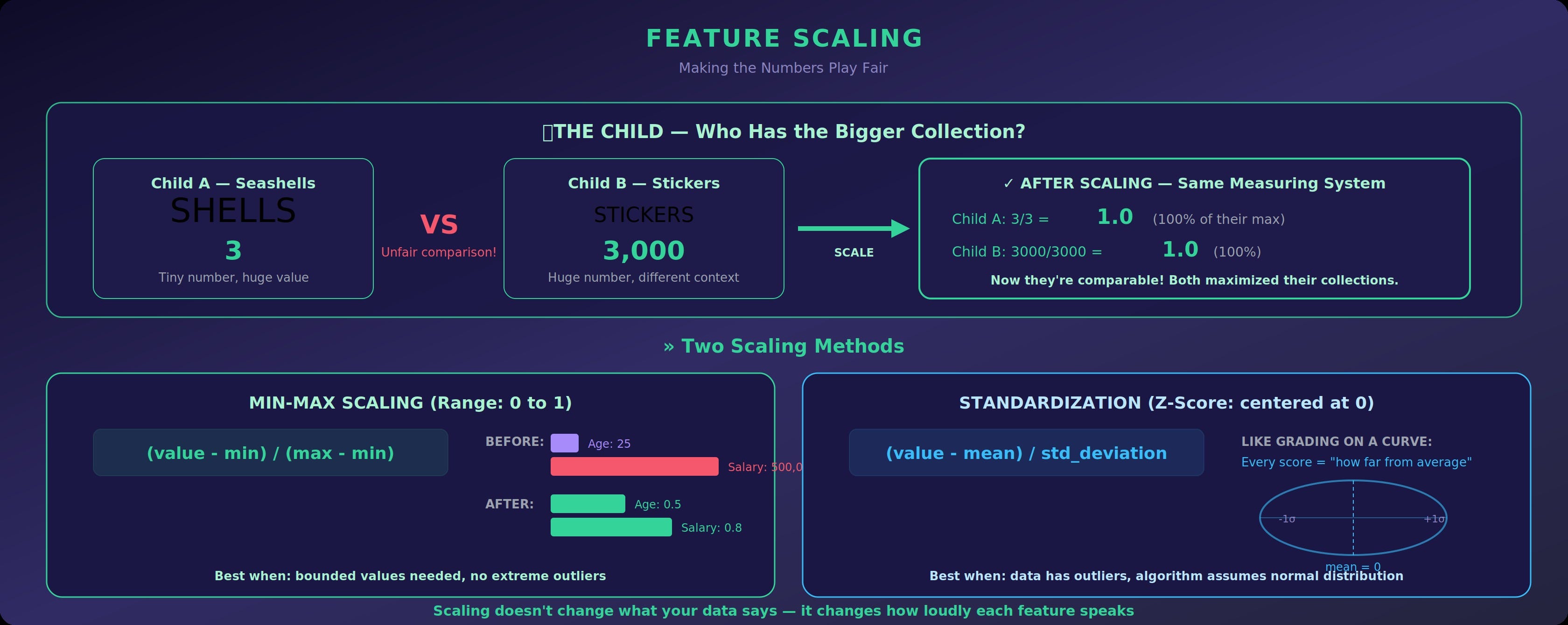
The Child: Imagine two children comparing their collections. One child has 3 seashells. The other has 3,000 stickers. If you ask, “Who has the bigger collection?” the answer seems obvious, but is it fair? The scales are completely different. To compare meaningfully, you’d need to put both collections on the same measuring system.
The Machine: ML models that calculate distances or gradients (like KNN, SVM, or neural networks) are heavily influenced by the magnitude of numbers. A feature ranging from 0 to 1,000,000 will dominate a feature ranging from 0 to 1, even if the smaller feature is more important.
Why it matters: Without scaling, large-magnitude features bully small-magnitude features into irrelevance. The model doesn’t know that “salary in rupees” and “years of experience” should carry equal weight; it just sees big numbers and small numbers.
The Two Main Scaling Methods
Min-Max Scaling (Normalization to a range): Squishes all values into a fixed range, typically 0 to 1. The formula: (value - min) / (max - min). Like converting both children’s collections to a percentage of their personal maximum. Works well when you need bounded values and your data doesn’t have extreme outliers.
Standardization (Z-score Scaling): Centers the data around 0 with a standard deviation of 1. The formula: (value - mean) / standard_deviation. Like grading on a curve — every student’s score is expressed as “how far from average.” Works well when your data has outliers or when your algorithm assumes normally distributed data.
The Takeaway: Scaling doesn’t change what your data says. It changes how loudly each feature speaks, so no single feature drowns out the others.
4. Normalization:
Reshaping the Distribution
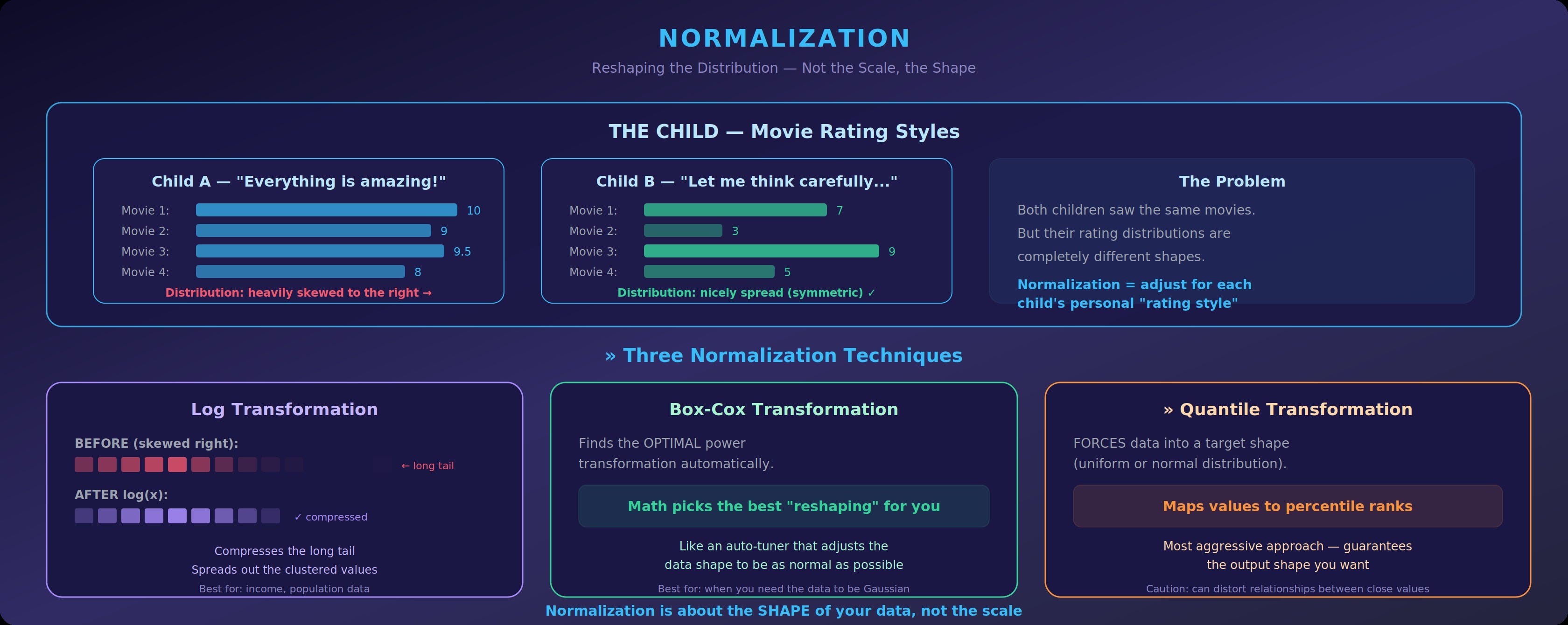
The Child: A teacher asks the class to rate how much they liked a movie on a scale of 1 to 10. One child always gives everything a 9 or 10. Another child’s ratings spread evenly from 1 to 10. To compare their opinions fairly, you’d need to adjust for each child’s personal rating style and their distribution.
The Machine: Normalization transforms the shape of your data’s distribution. Even after scaling, your data might be heavily skewed, with most values clustered on one side with a long tail. Many ML algorithms perform better when the data follows a more symmetric, bell-curve-like distribution.
Why it matters: Skewed distributions can mislead models. If 95% of your income data clusters between ₹20,000 and ₹80,000 but a few values shoot up to ₹50,00,000, the model might overfit to those extremes or underperform on the majority.
Common Normalization Techniques
Log Transformation: Take the logarithm of each value. This compresses the long tail and spreads out the clustered values. Extremely effective for income data, population data, or anything with exponential growth patterns.
Box-Cox Transformation: A more flexible version that finds the optimal power transformation to make your data as close to a normal distribution as possible. The math picks the best “reshaping” automatically.
Quantile Transformation: Forces the data into a specific distribution (usually uniform or normal) by mapping values to their percentile ranks. The most aggressive approach guarantees the output shape but can distort relationships between close values.
The Takeaway: Normalization is about the shape of your data, not the scale. It ensures your data’s distribution doesn’t secretly sabotage your model’s assumptions.
Scaling vs. Normalization:
Clearing Up the Confusion
These two terms get mixed up constantly,
Scaling adjusts the range or magnitude of your features. It answers: “How big are these numbers relative to each other?”
Normalization adjusts the distribution shape of your features. It answers: “What does the spread of these numbers look like?”

You often need both. Scale first to get features on comparable ranges, then normalize if the distribution is skewed.
Think of it as: scaling sets the volume, normalization tunes the equalizer.
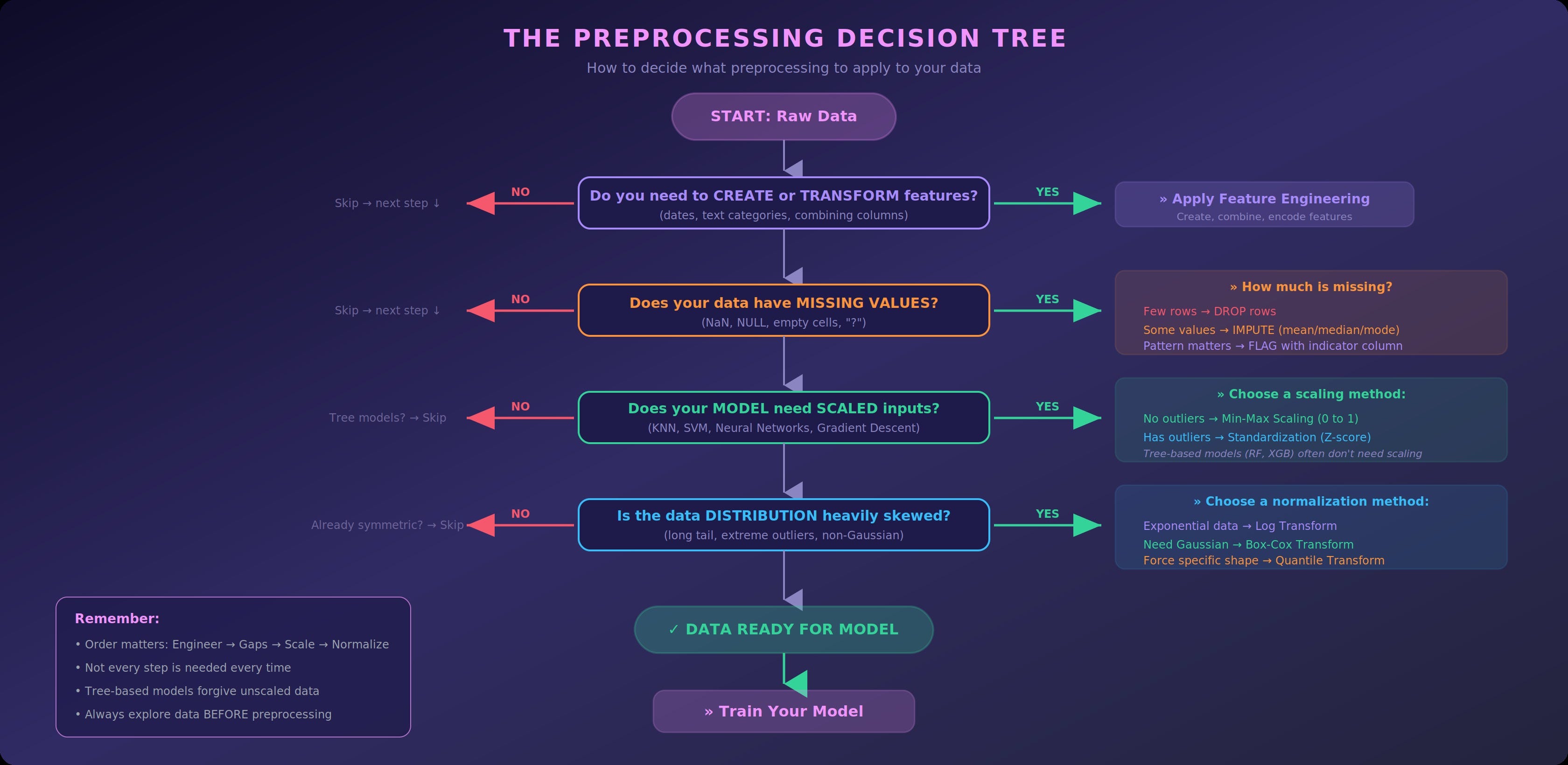
The Preprocessing Decision Tree
How do you decide what preprocessing to apply?
Conclusion
Data preprocessing isn’t glamorous. Nobody writes headlines about it. But it is, without exaggeration, where most real ML work happens.
Feature engineering decides what the model gets to see. Missing value handling decides how gaps are managed. Scaling ensures no feature unfairly dominates. Normalization reshapes distributions so algorithms can work as designed.
These aren’t optional steps you can skip when you’re in a hurry. They’re the foundation. Every model, every prediction, every result sits on top of how well you prepared the data.
If you step back, the pattern is strikingly familiar: whether it’s a child learning to organize their toy box or a model learning to classify images, the quality of learning depends entirely on the quality of preparation.
Get the data right, and the model will surprise you. Skip the preparation, and no algorithm in the world will save you.